DIFFUSION FROM SCRATCH
A denoising diffusion model (DDPM) written in ~250 lines of plain PyTorch and trained on CIFAR-10 — no diffusers library, no pretrained weights, no hidden machinery. It learns to turn static into tiny photographs, and the whole network exports to ONNX so it can eventually run right here in your browser.
Destroy, then learn to undo
Diffusion models are built on a trick that sounds backwards: the only thing the network ever learns is how to clean up noise.
1 · FORWARD: DROWN THE IMAGE
Take a real photo and add a little Gaussian noise, 1000 times, following a fixed schedule (β ramps linearly from 1e-4 to 0.02). By the end nothing survives — it's TV static. The useful part: you never have to noise step-by-step. A closed-form shortcut jumps straight to any timestep t.
x_t = √ᾱ·x₀ + √(1−ᾱ)·ε2 · LEARN: GUESS THE NOISE
The training loop is almost embarrassingly simple: pick a photo, pick a random t, noise it with the shortcut, and ask a U-Net — which sees the noisy image plus an embedding of t — to predict exactly which noise was added. The loss is plain MSE between the guess and the truth. That's it. Repeated 117,000 times, that one task forces the network to learn what images look like.
3 · SAMPLE: RUN IT BACKWARDS
To generate, start from pure noise and repeatedly ask the network "what noise is in this?" — subtract its estimate to get a guess at the clean image, re-noise to a slightly earlier timestep, and repeat. DDIM makes this deterministic and takes 50 strides instead of 1000 steps. An image no one has ever seen condenses out of static.
"From scratch" here means every piece — the U-Net, the noise schedule, the timestep embeddings, EMA weight averaging, mixed-precision training, the DDIM sampler — is written out by hand in train_diffusion.py, following the original DDPM paper (Ho et al., 2020) rather than importing a library that hides it.
Six moving parts
Everything below ships in four small Python files. Numbers are from the actual training run, not a spec sheet.
DATASET — CIFAR-10
50,000 tiny 32×32 photos in 10 classes. Random horizontal flips, pixels normalized to [−1, 1], batches of 128 (390 batches per epoch). Small enough to train honestly on one consumer GPU.
NOISE SCHEDULE — LINEAR β, T=1000
β ramps from 1e-4 to 0.02 across 1000 timesteps; ᾱ_t is precomputed as the cumulative product of (1−β). Charted for real below.
U-NET — 18.7M PARAMETERS
Three resolution levels (32→16→8) with 128/256/256 channels, residual blocks fed sinusoidal timestep embeddings, self-attention at 16² and 8², GroupNorm + SiLU, dropout 0.1. Skip connections carry fine detail across the bottleneck.
TRAINING LOOP — PREDICT ε, MSE LOSS
Adam at 2e-4 with AMP mixed precision; an EMA copy of the weights (decay 0.9995) is what actually generates. 300 epochs ≈ 117k steps, about 4 hours on a single RTX 3090, final loss ≈ 0.029. Checkpoints are resumable.
SAMPLER — DDIM, 50 STEPS
Deterministic sampling: at each of 50 timesteps the model predicts the noise, the loop reconstructs a clamped estimate of x₀, then re-noises it to the next timestep down. 20× fewer steps than naive DDPM sampling with no perceptible quality loss at this scale.
ONNX EXPORT — BROWSER-READY
export_onnx.py exports the EMA U-Net at opset 17 (75 MB) and verifies it against PyTorch to <1e-3 max abs difference. ONNX Runtime Web runs it on WebGPU — a 50-step sample takes about 2 seconds client-side, with a WASM fallback.
Two curves that explain everything
The schedule decides how fast images drown; the loss curve shows why you should never trust it as a progress bar.
Computed, not sketched: this is the exact schedule from train_diffusion.py— β linear from 1e-4 to 0.02 over T=1000, ᾱt= ∏(1−β). By t≈350 less than half the signal survives; by t=999 only 0.004% does. The mustard dots are the 50 timesteps DDIM actually visits when sampling.
Representative curve— per-epoch losses were printed to console during the run, not logged to disk. The anchors are real: loss collapses to ≈0.03 within about five epochs and the run finished at ≈0.029. The honest lesson: for diffusion, loss is a nearly useless progress signal — it flatlines while the samples below keep improving for another 295 epochs. Judge by the grids.
Watching a model learn to see
Uncurated 8×8 grids sampled from the same training run as it progressed — every grid is DDIM, 50 steps, EMA weights. No cherry picking.
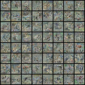
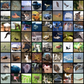
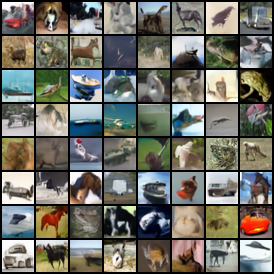
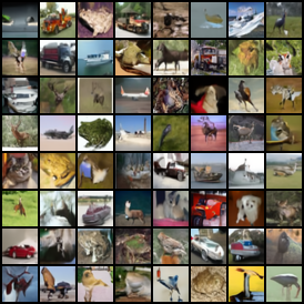
Between epoch 10 and epoch 300 the training loss moved by roughly 0.002. The images did not get the memo — which is exactly the point made by the loss chart above.
Scrub the trajectory yourself
Real samples from the trained model, real schedule math, one honest shortcut — the fine print is under the panel.
- timestep t
- 999 / 999
- ᾱ_t (signal kept)
- 0.0000
- √(1−ᾱ) (noise)
- 1.000
What's real: the pixels (samples from the trained model), the ᾱ schedule, and the 50-step trajectory GENERATE walks through. What's simulated:the denoising itself — this scrubber renders the closed-form forward process q(x_t | x₀) in reverse rather than running the U-Net 50 times. Want the real thing? The network is exported to ONNX and deployed — it samples live on WebGPU at the demo Space ↗. Bringing that loop onto this page is the roadmap item below.
Ledger
unet.onnx on the Hub ↗.